YOLO是“You Only Look Once”的缩写,YOLO将物体检测作为回归问题求解,是一个对象检测算法的名字,这是Redmon等人在2016年的一篇研究论文中命名的。

本篇文章会一步一步搭建起yolov3的神经网络,详细内容会具体分析。
YOLO介绍
目标检测(object detection)是一个因近年来深度学习的发展而受益颇多的领域,近年来,人们开发了多种目标检测算法,其中包括YOLO、SSD、Mask-RCNN和RetinaNet。此篇文章使用PyTorch并基于YOLO v3来实现一个目标检测器,这是一种速度更快的目标检测算法。
YOLO是“You Only Look Once”的缩写,YOLO将物体检测作为回归问题求解,是一个对象检测算法的名字,这是Redmon等人在2016年的一篇研究论文中命名的:
Redmon J , Divvala S , Girshick R , et al. You Only Look Once: Unified, Real-Time Object Detection[J]. 2015.
YOLO结构
以下为yolo的整体结构:
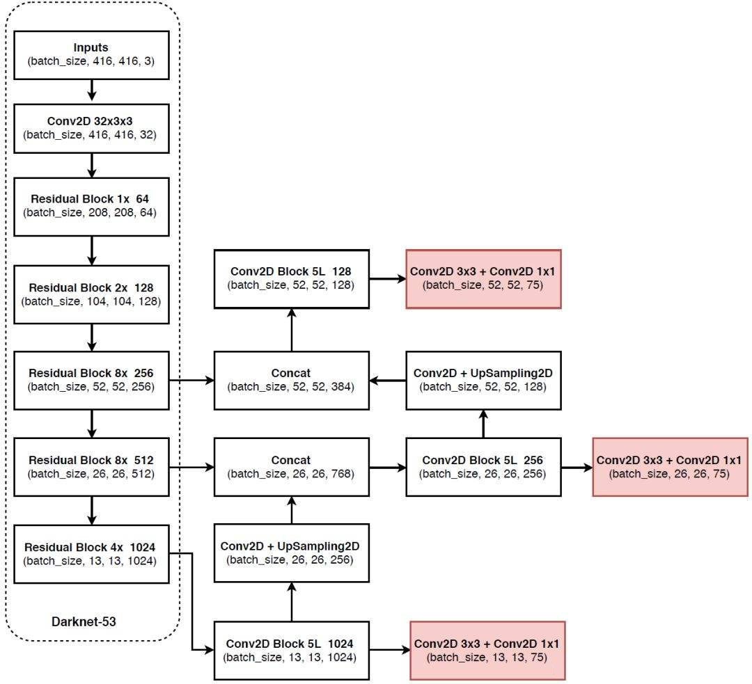
这张图分成两部分,左边虚线框起来的是主干特征提取部分。
主干特征提取
这部分称作Darknet-53,主干特征提取顾名思义,用来提取图片的特征。
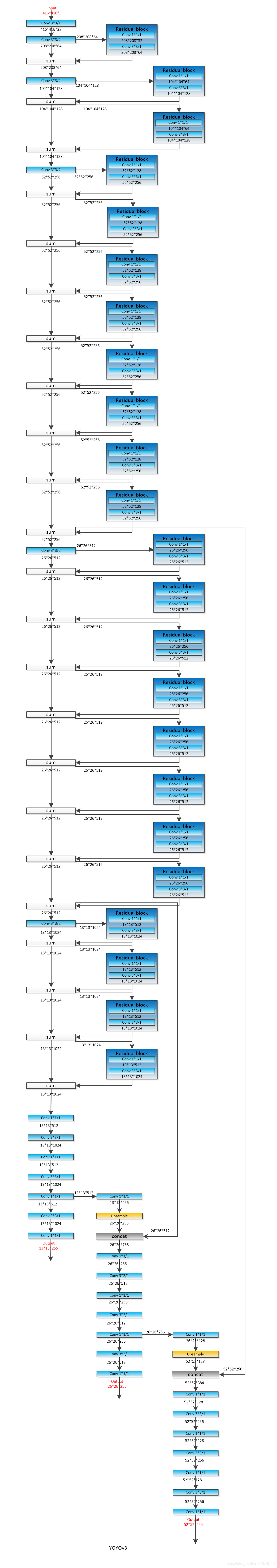
输入是需要一张$416 416 3$大小的图片,然后是不断卷积的过程,如果仔细看会发现图片的高和宽不断被压缩,通道数却不断扩张,这是一个下采样过程。
经过下采样之后,会获得特征层(用来表述图片的特征),下图是我们需要的特征层。
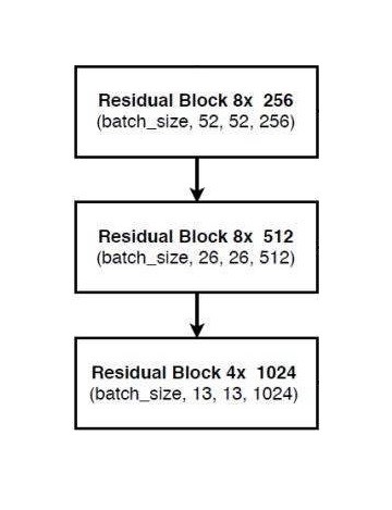
由此可见保留下来的特征层为:$5252256$、$2626512$、$13131024$三种尺寸,这三种特征层是即将传入右边的部分。
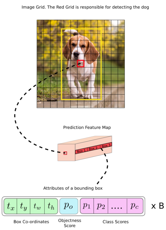
每个特征图可以看作一个“条目”,因为一个“条目”有一些信息,如下图所示:
其他部分
这里的其他部分泛指右边部分的网络。
经过主干特征提取后,我们获得了三种尺寸的特征层,分别对三种尺寸的特征层处理。
处理$13131024$特征层
首先说一下$13131024$特征层的处理:
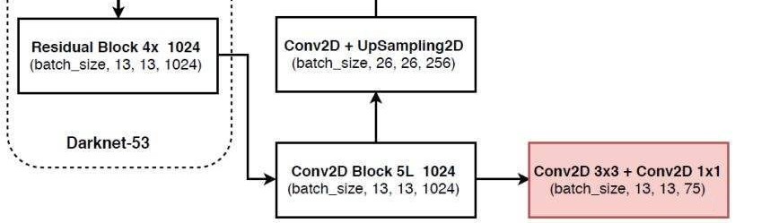
可以看到$13131024$特征层经过了5次卷积后传到了两个方向。
右边的粉色部分是分类预测和回归预测,其实就是两次卷积,最后会获得$131375$大小的,再经过一个分解变成$1313325$,即$13133(20 + 1 + 4)$,这个过程其实就是化成$1313$的网格,每个网格有3个预测出的*先验框,接下来会根据判断属于那种框的尺寸。
之所以会把25分成三部分,其实就gailv是20个物体分类,由于使用voc数据集,所以会有20个,coco训练集会出现80个,简单来讲20个置信度(属于哪个类的概率)会分类属于哪个类;1是指是否有物体;4是对框的调整。
注意$13131024$特征层还有一个传递方向,这时需要一个上采样,也就是扩增长宽,减小通道数。经过上采样之后会和$2626512$特征层进行堆叠(增加通道数)。
处理$2626512$特征层
$2626512$特征层在和经过上采样的$13131024$特征层进行堆叠后,会形成一个新的“特征金字塔”,当然这个特征金字塔还会继续堆叠。
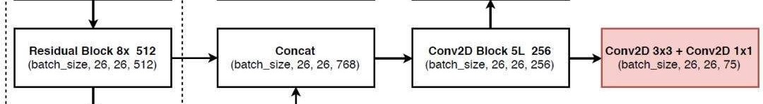
后面的部分就一样了,再5次卷积,在最后进行分类预测和回归预测,会出现相同操作。
与此同时会把5次卷积后继续向上传递,并有个上采样。
$5252256$特征层同样如此就不再赘述。
输出结果:
$t_x$和$t_y$是被检测物体的中心位置,$t_w$和$t_h$是方框的尺寸,$p_0$是物体置信度,代表了这个区域内有物体的概率,$p_1->p_c$是分类置信度,哪类概率高,就属于什么物体。最后还有个B,这个是锚框个数,说明了这个区域可以最多检测出B个物体。
Anchor Boxes
有的翻译成锚框,有的翻译成先验框,这里我就叫它锚框了。
YOLO不能直接预测边界框的宽度和高度,这会导致训练过程中出现不稳定的变化。大多数现代目标检测器会预测对数空间转换,或者只是偏移到称为锚点的预定义默认锚框。YOLO-v3具有三个锚点,可在每个细胞单元格上预测三个边界框。
那么真正的方框是怎么预测出的?先看下面的公式:
前两个公式是预测中心点,经过$\sigma()$函数后就会稳定在0和1之间。$c_x$和$c_y$是第几个方框,例如上图中红色框的这两值都是6。
后面两个公式预测宽度,$p_w$和$p_h$是锚框的尺寸,直接乘就可以。
还没有完,这只完成了一半,接着看:
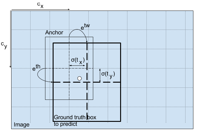
中心点需要还乘上对应的网格宽度,方框需要带入e指数中。
补一张更漂亮的图。
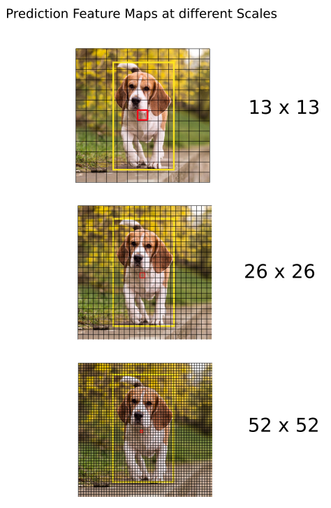
YOLO预测原理
YOLO将图片分成了3种检测,检测的区别是按照分割区域的大小。
首先输入图片的大小要定下为$416*416$大小,如果不合适就要补上缺失部分,目的就是防止失真。
将图片分别分成$5252$、$2626$、$13*13$、三种尺寸的网格,针对的识别三种尺寸,也就对应上了上部分的三种输出结果。
每个输出结果的维度为(N, 75 * 3, x, x),x为尺寸分别对应52、26、13三种,N代表样本数,75 * 3这个数在上面提过了就不再多说。
最后的最终的预测结构后还要进行得分排序与非极大抑制筛选。
用$77$来举例(我只找到$77$的例子,我又懒得去做$1313$的图),下面将一幅图分成$77$网格,共49部分。
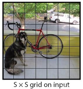
对于每个网格点,都会预测一个边界框和与每个类别(汽车,行人,交通信号灯等)相对应的概率,每个网络点负责一个区域的检测。
程序
首先搭建DarkNet大概框架:
1
2
3
| class DarkNet(nn.Module):
def __init__(self, layers):
super(DarkNet, self).__init__()
|
DarkNet继承了pytorch中的模型,目的使用一些相同的框架函数。
初始的卷积层
继续根据整体结构来加入每一层,首先卷积层:
1
2
3
4
5
6
|
self.inplanes = 32
self.conv1 = nn.Conv2d(3, self.inplanes, kernel_size=3, stride=1, padding=1, bias=False)
|
标准化和激活函数:
注意:这里使用的是LeakyReLU,这样好处是,负数区域还存在值,同时也有斜率。
1
2
3
4
|
self.bn1 = nn.BatchNorm2d(self.inplanes)
self.relu1 = nn.LeakyReLU(0.1)
|
以上操作建立了一个卷积层,最后生成的维度为:(N, 416, 416, 32)
残差块
先制做出残差块的函数,返回值是一个残差块:
1
2
3
4
5
6
7
8
9
10
11
12
13
14
15
16
17
18
19
20
21
22
23
24
25
26
27
28
29
| def _make_layer(self, planes, blocks):
"""
制作一个结构块
:param planes: 是个列表,第一位置是输入通道数,第二位置是输出通道数
:param blocks: 残差块堆叠个数
:return:
"""
layers = []
layers.append(("ds_conv", nn.Conv2d(self.inplanes, planes[1], kernel_size=3,
stride=2, padding=1, bias=False)))
layers.append(("ds_bn", nn.BatchNorm2d(planes[1])))
layers.append(("ds_relu", nn.LeakyReLU(0.1)))
self.inplanes = planes[1]
for i in range(0, blocks):
layers.append(("residual_{}".format(i), BasicBlock(self.inplanes, planes)))
return nn.Sequential(OrderedDict(layers))
|
OrderedDict是有序字典,虽然平常不常用,但在这里使用是最合适的,记得导入包:
1
| from collections import OrderedDict
|
最核心的部分是BasicBlock类,这里是残差网络相加的地方:
1
2
3
4
5
6
7
8
9
10
11
12
13
14
15
16
17
18
19
20
21
22
23
24
25
26
27
28
29
30
31
32
33
34
35
36
37
38
39
40
41
42
43
44
45
46
47
48
|
class BasicBlock(nn.Module):
def __init__(self, inplanes, planes):
"""
残差块
:param inplanes:
:param planes: 下采样部分
"""
super(BasicBlock, self).__init__()
self.conv1 = nn.Conv2d(inplanes, planes[0], kernel_size=1,
stride=1, padding=0, bias=False)
self.bn1 = nn.BatchNorm2d(planes[0])
self.relu1 = nn.LeakyReLU(0.1)
self.conv2 = nn.Conv2d(planes[0], planes[1], kernel_size=3,
stride=1, padding=1, bias=False)
self.bn2 = nn.BatchNorm2d(planes[1])
self.relu2 = nn.LeakyReLU(0.1)
def forward(self, x):
residual = x
out = self.conv1(x)
out = self.bn1(out)
out = self.relu1(out)
out = self.conv2(out)
out = self.bn2(out)
out = self.relu2(out)
out += residual
return out
|
由于里面先进行1卷积,再3卷积,这样可以减少参数量,
初始化剩下的东西:
1
2
3
4
5
6
7
8
9
10
11
|
self.layers_out_filters = [64, 128, 256, 512, 1024]
for m in self.modules():
if isinstance(m, nn.Conv2d):
n = m.kernel_size[0] * m.kernel_size[1] * m.out_channels
m.weight.data.normal_(0, math.sqrt(2. / n))
elif isinstance(m, nn.BatchNorm2d):
m.weight.data.fill_(1)
m.bias.data.zero_()
|
前向传播
前向传播的时候我们需要返回三个尺寸的特征图,所以需要这样写:
1
2
3
4
5
6
7
8
9
10
11
12
13
14
15
16
17
18
19
20
21
22
23
| def forward(self, x):
"""
前向传播
:param x: 输入图
:return: 三个特征图
"""
x = self.conv1(x)
x = self.bn1(x)
x = self.relu1(x)
x = self.layer1(x)
x = self.layer2(x)
out3 = self.layer3(x)
out4 = self.layer4(out3)
out5 = self.layer5(out4)
return out3, out4, out5
|
从特征获取预测结果
特征图出来了,但我们需要将特征图转换成最终结果。
在放代码之前,自定义一套卷积,这是方便后面快速使用:
1
2
3
4
5
6
7
8
9
10
11
12
13
14
| def conv2d(filter_in, filter_out, kernel_size):
"""
私自定义的卷积
:param filter_in: 输入通道数
:param filter_out: 输出通道数
:param kernel_size: 卷积核尺寸
:return:
"""
pad = (kernel_size - 1) // 2 if kernel_size else 0
return nn.Sequential(OrderedDict([
("conv", nn.Conv2d(filter_in, filter_out, kernel_size=kernel_size, stride=1, padding=pad, bias=False)),
("bn", nn.BatchNorm2d(filter_out)),
("relu", nn.LeakyReLU(0.1)),
]))
|
这个卷积相当于一套完整的卷积层,但官方这里没有使用残差网络,这有点让我感到疑惑,因为我担心这样会不会影响整个网络前部分的梯度计算。
主体部分的初始化
因为是主体部分,所以首先创建yolo主体:
1
2
3
4
5
6
7
8
| class YoloBody(nn.Module):
def __init__(self, config):
"""
yolo主体
:param config:
"""
super(YoloBody, self).__init__()
self.config = config
|
然后获取已经创建好的网络(也就是上面的程序):
1
2
3
4
5
|
self.backbone = darknet53(None)
out_filters = self.backbone.layers_out_filters
|
接下来就是$13*13$特征层的提取:
1
2
3
4
5
6
|
final_out_filter0 = len(config["yolo"]["anchors"][0]) * (5 + config["yolo"]["classes"])
self.last_layer0 = make_last_layers([512, 1024], out_filters[-1], final_out_filter0)
|
现在详细说一下final_out_filter0这个变量特点,此变量分两部分,两部分相乘才出结果。len(config["yolo"]["anchors"][0])是先验框个数,我们使用了3个,所以此结果是3;(5 + config["yolo"]["classes"])这个是$20 + 1 + 4$,也就是25。最终结果就是$(20+1+4)*3=75$。
这个时候有个make_last_layers函数,这就是5次卷积和最后结果卷积。
1
2
3
4
5
6
7
8
9
10
11
12
13
14
15
16
17
18
19
20
21
22
23
24
25
26
| def make_last_layers(filters_list, in_filters, out_filter):
"""
5次卷积+2次卷积
:param filters_list:中间过渡通道数
:param in_filters: 输入通道数
:param out_filter: 输出通道数
:return: 5次卷积+2次卷积的模型
"""
m = nn.ModuleList([
conv2d(in_filters, filters_list[0], 1),
conv2d(filters_list[0], filters_list[1], 3),
conv2d(filters_list[1], filters_list[0], 1),
conv2d(filters_list[0], filters_list[1], 3),
conv2d(filters_list[1], filters_list[0], 1),
conv2d(filters_list[0], filters_list[1], 3),
nn.Conv2d(filters_list[1], out_filter, kernel_size=1,
stride=1, padding=0, bias=True)
])
return m
|
$1*1$卷积是很有效减少通道数,从而减少参数,这对电脑减轻了不小负担。
接下来是$13*13$特征层的提取:
1
2
3
4
5
6
7
8
9
|
final_out_filter1 = len(config["yolo"]["anchors"][1]) * (5 + config["yolo"]["classes"])
self.last_layer1_conv = conv2d(512, 256, 1)
self.last_layer1_upsample = nn.Upsample(scale_factor=2, mode='nearest')
self.last_layer1 = make_last_layers([256, 512], out_filters[-2] + 256, final_out_filter1)
|
在使用上采样之前需要用$1*1$卷积核来调整通道,这样可以保证接下来上采样时通道一致。
由于使用上采样,所以我们需要上采样函数,幸运的是pytorch提供了上采样,所以我们免去了这个过程。
最后就是剩下特征层,也是同样道理:
1
2
3
4
5
6
7
8
9
|
final_out_filter2 = len(config["yolo"]["anchors"][2]) * (5 + config["yolo"]["classes"])
self.last_layer2_conv = conv2d(256, 128, 1)
self.last_layer2_upsample = nn.Upsample(scale_factor=2, mode='nearest')
self.last_layer2 = make_last_layers([128, 256], out_filters[-3] + 128, final_out_filter2)
|
前向传播
看到这里,所有初始化都完成了,也就是网络结构部分完成了,剩下就是其他的代码,就比如前向传播的整体还没写。
1
2
3
4
5
6
7
8
9
10
11
12
13
14
15
16
17
18
19
20
21
| def forward(self, x):
"""
前向传播
:param x: 输入
:return:
"""
def _branch(last_layer, layer_in):
"""
分开卷积过程
:param last_layer: 上一层结果
:param layer_in:会存入卷积过程的结果并会返回出去
:return: out_branch是最后结果
"""
for i, e in enumerate(last_layer):
layer_in = e(layer_in)
if i == 4:
out_branch = layer_in
return layer_in, out_branch
|
没错,直接套娃就可以,我挺喜欢这样写,因为这样写可以让整个函数在另一个函数周期里,外函数“死亡”时,里面的函数也会“死亡”。之所以定义这个函数是把第五次卷积结果拿出来,因为需要上采样传递给其他层。
继续写,在DarkNet中我们可以获得到三种特征图。
1
2
|
x2, x1, x0 = self.backbone(x)
|
现在可以正常正向传播了,首先第一套特征图:
1
2
3
|
out0, out0_branch = _branch(self.last_layer0, x0)
|
第二套特征图使用计算之前,需要调整通道数、上采样、堆叠:
1
2
3
4
5
6
7
8
9
|
x1_in = self.last_layer1_conv(out0_branch)
x1_in = self.last_layer1_upsample(x1_in)
x1_in = torch.cat([x1_in, x1], 1)
out1, out1_branch = _branch(self.last_layer1, x1_in)
|
第三套同样如此:
1
2
3
4
5
6
7
8
9
|
x2_in = self.last_layer2_conv(out1_branch)
x2_in = self.last_layer2_upsample(x2_in)
x2_in = torch.cat([x2_in, x2], 1)
out2, _ = _branch(self.last_layer2, x2_in)
|
最后直接输出:
以上我们的网络就搭建完毕了,但还缺少解码部分以及损失函数,所以继续写吧。
解码
将解码也定义一个层,这样就方便后续的处理:
1
2
3
4
5
6
7
8
9
| class DecodeBox(nn.Module):
def __init__(self, anchors, num_classes, img_size):
super(DecodeBox, self).__init__()
self.anchors = anchors
self.num_anchors = len(anchors)
self.num_classes = num_classes
self.bbox_attrs = 5 + num_classes
self.img_size = img_size
|
前向传播部分:
1
2
3
4
5
6
7
8
9
10
11
| def forward(self, input):
batch_size = input.size(0)
input_height = input.size(2)
input_width = input.size(3)
|
当然还没完,我们还要获得图片步长,也就是图片每个网格内有多少像素点(感受野):
1
2
3
4
5
|
stride_h = self.img_size[1] / input_height
stride_w = self.img_size[0] / input_width
|
我们之前定义了三种先验框,所以注意最开始的先验框的单位是像素,我们需要将这个改变成根据步长的百分比,也就是归一到特征层上:
1
2
|
scaled_anchors = [(anchor_width / stride_w, anchor_height / stride_h) for anchor_width, anchor_height in self.anchors]
|
因为有三套先验框,所以这个循环会执行三次。
还需要通道转换,.permute(0, 1, 3, 4, 2).contiguous():
1
2
3
|
prediction = input.view(batch_size, self.num_anchors,
self.bbox_attrs, input_height, input_width).permute(0, 1, 3, 4, 2).contiguous()
|
处理一下先验框的中心参数,怕是遇到负数,所以使用sigmoid()函数过滤一下,这样百分百是正数且不会大于1:
1
2
3
|
x = torch.sigmoid(prediction[..., 0])
y = torch.sigmoid(prediction[..., 1])
|
还有宽高参数:
1
2
3
|
w = prediction[..., 2]
h = prediction[..., 3]
|
以及物体置信度和种类置信度,听说在之前yolo使用的是softmax()函数,这样就会产生独立事件,有时会出bug,sigmoid()可以解决这个问题:
1
2
3
4
|
conf = torch.sigmoid(prediction[..., 4])
pred_cls = torch.sigmoid(prediction[..., 5:])
|
先验框问题解决了,接下来就生成出来,根据网格左上角生成中心:
1
2
3
|
grid_x = torch.linspace(0, input_width - 1, input_width).repeat(input_width, 1).repeat(batch_size * self.num_anchors, 1, 1).view(x.shape).type(FloatTensor)
grid_y = torch.linspace(0, input_height - 1, input_height).repeat(input_height, 1).t().repeat(batch_size * self.num_anchors, 1, 1).view(y.shape).type(FloatTensor)
|
也就是从网格的左上角,每隔size单位生成一个,形状是(N, 3, size, size)
再生成先验框的宽和高,根据自己设定的原始先验框:
1
2
3
4
5
|
anchor_w = FloatTensor(scaled_anchors).index_select(1, LongTensor([0]))
anchor_h = FloatTensor(scaled_anchors).index_select(1, LongTensor([1]))
anchor_w = anchor_w.repeat(batch_size, 1).repeat(1, 1, input_height * input_width).view(w.shape)
anchor_h = anchor_h.repeat(batch_size, 1).repeat(1, 1, input_height * input_width).view(h.shape)
|
这是最后的调整了:
1
2
3
4
5
6
|
pred_boxes = FloatTensor(prediction[..., :4].shape)
pred_boxes[..., 0] = x.data + grid_x
pred_boxes[..., 1] = y.data + grid_y
pred_boxes[..., 2] = torch.exp(w.data) * anchor_w
pred_boxes[..., 3] = torch.exp(h.data) * anchor_h
|
之前我们获得的先验框中心是一个0到1之间的数字,加上网格的次序就可以直接检查出是哪个网格中的中心。
结尾:
1
2
3
4
|
_scale = torch.Tensor([stride_w, stride_h] * 2).type(FloatTensor)
output = torch.cat((pred_boxes.view(batch_size, -1, 4) * _scale,conf.view(batch_size, -1, 1), pred_cls.view(batch_size, -1, self.num_classes)), -1)
return output.data
|
参考:
https://blog.csdn.net/weixin_44791964/article/details/105310627
https://www.bilibili.com/video/BV1Hp4y1y788
 微信
微信 支付宝
支付宝